DHS Data Wrangling and Analysis

I requested DHS data for Zambia (2018, DHS-VII).

Import the households dataset for your selected country and create a data frame with a variable that describes each of the following: household ID, unit, weights, location, size, gender, age, education, and wealth.

In this case, after looking at the .MAP and .DO files, province was the best option to describe location.

households <- read_dta("ZM_2018_DHS/ZMHR71DT/ZMHR71FL.DTA")

hhid <- households$hhid #check length(unique(hhid))
unit <- households$hv004                 #ultimate area unit
weights <- households$hv005 / 1000000    #household sample weight (6 decimals)
location <- as_factor(households$hv024)  #province
size <- households$hv009                 #number of household members
sex <- households[ ,282:309]             #hv104_1 through hv104_28
age <- households[ ,310:337]             #hv105_1 through hv105_28
edu <- households[ ,338:385]             #hv106_1 through hv106_28

wealth <- households$hv270               #wealth index combined

hhs <- cbind.data.frame(hhid, unit, weights, location, size, sex, age, edu, wealth)

Pivot the persons columns within your households data to a long format in order to produce a similarly specified dataset that describes all persons residing within all households.

gender <- hhs %>%
  pivot_longer(cols = starts_with("hv104"),
               names_to = "pid",
               values_to = "gender",
               values_drop_na = TRUE)

age <- hhs %>%
  pivot_longer(cols = starts_with("hv105"),
               names_to = "pid",
               values_to = "age",
               values_drop_na = TRUE)

edu <- hhs %>%
  pivot_longer(cols = starts_with("hv106"),
               names_to = "pid",
               values_to = "edu",
               values_drop_na = TRUE)

Following pivoting and dropping NA, number of observations (specifically gender) was not equal, so utlized code (below) to merge columns.

gender$id <- paste(gender$hhid, substr(gender$pid, 7,8), sep = '')
age$id <- paste(age$hhid, substr(age$pid, 7,8), sep = '')
edu$id <- paste(edu$hhid, substr(edu$pid, 7,8), sep = '')

pns <- inner_join(gender, age, by = "id") %>% inner_join(., edu, by = "id")

Now, sum(pns$weights) gives us 40560.92, and nrow(pns) gives us 40777.

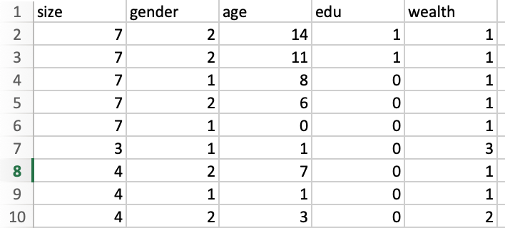
First few rows of pns dataframe:

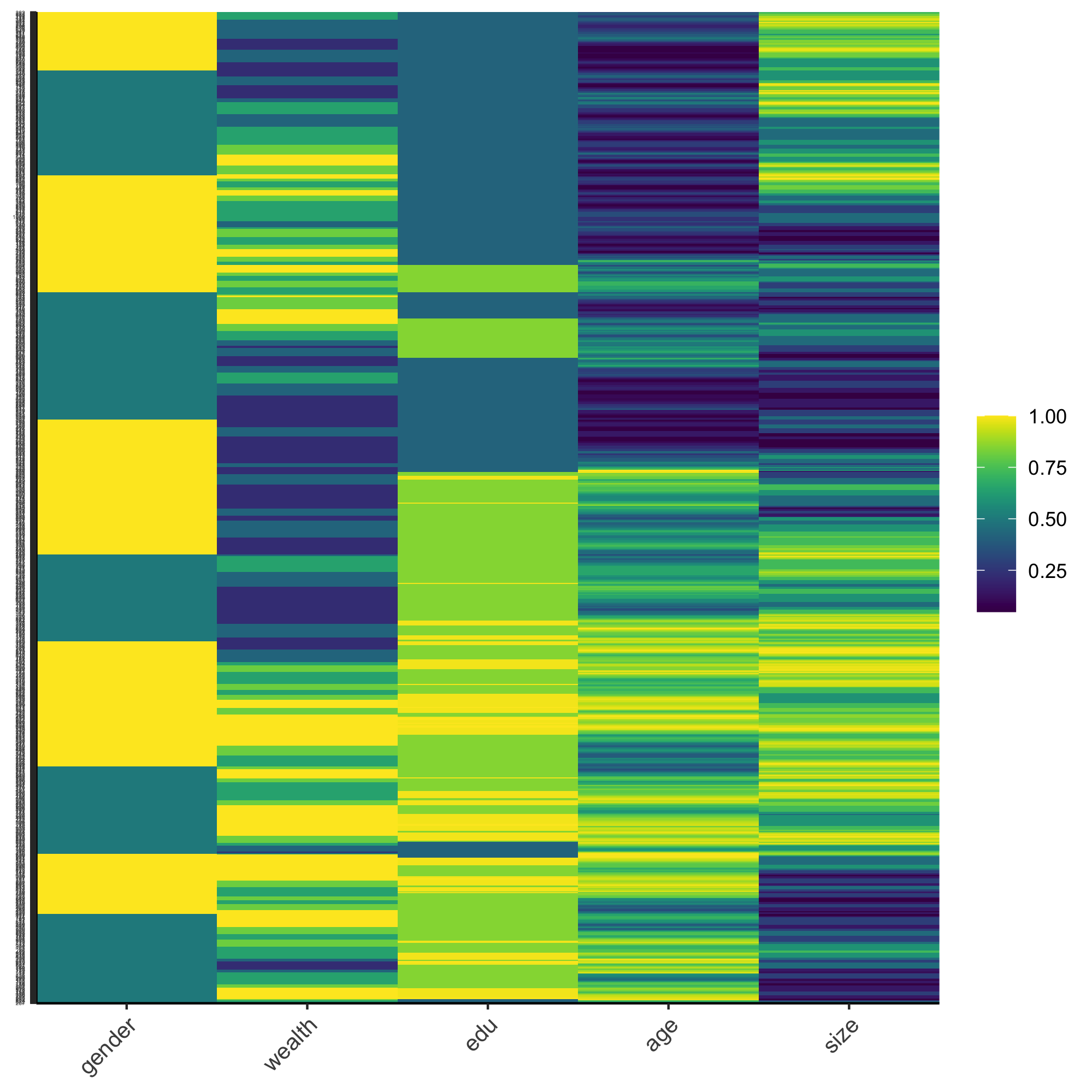
Using this data frame describing all persons standardize, normalize and percentize your variables and visualize each post transformed dataset as a heatmap that illustrates the heterogeneity of the combination of patterns.

Raw:

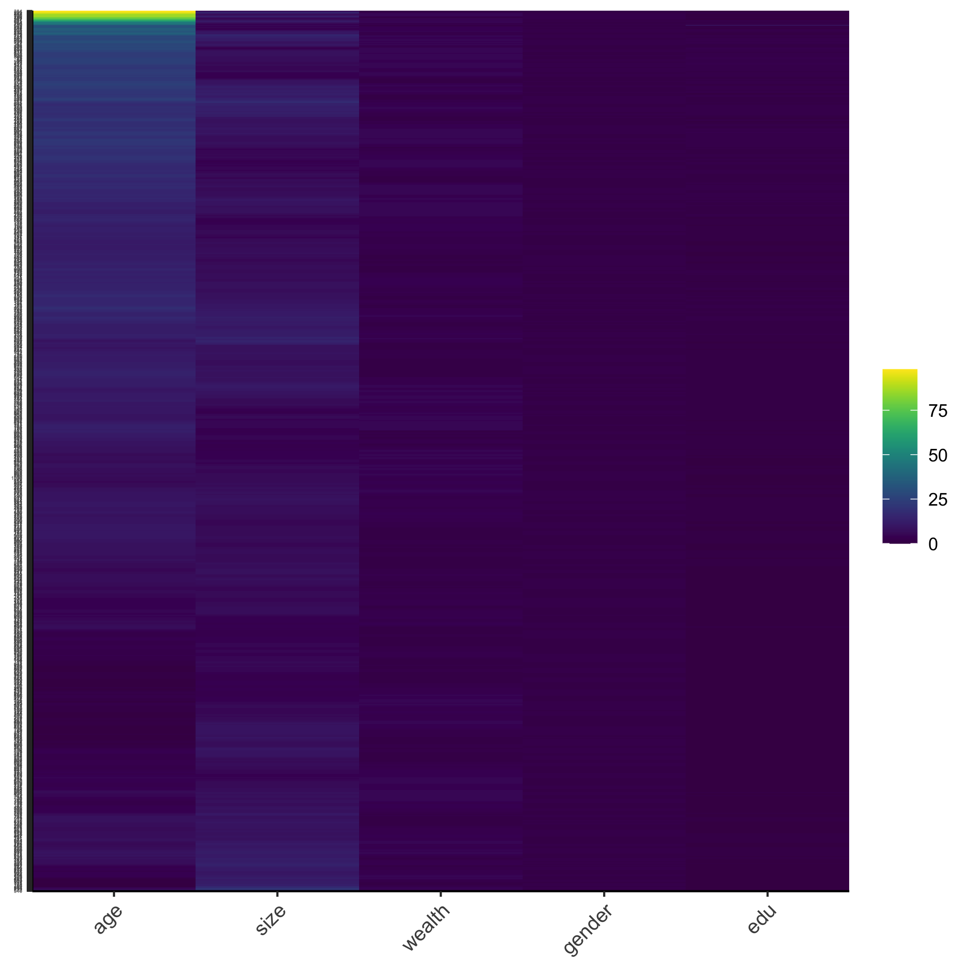
Standardized (scaled):

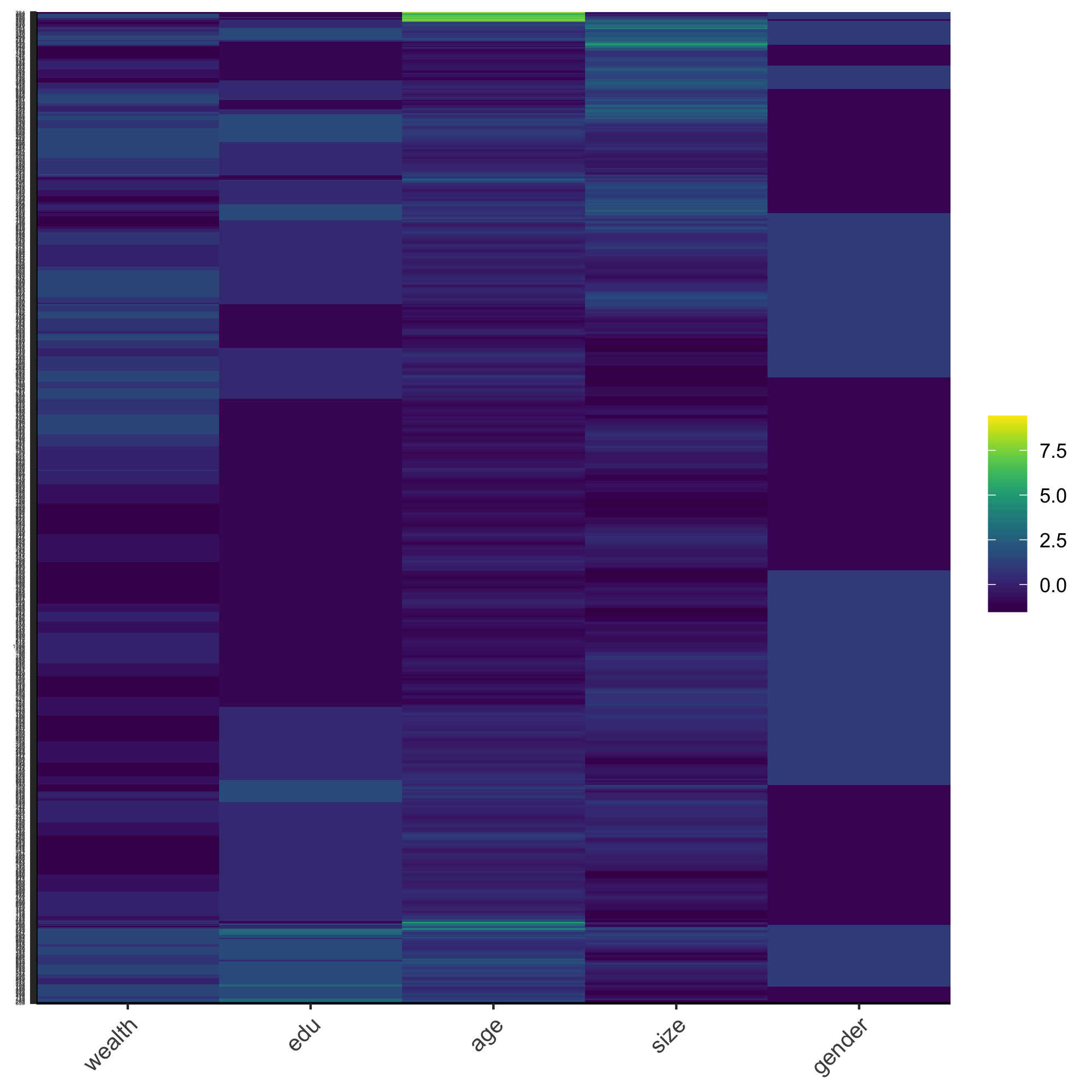
Normalized:

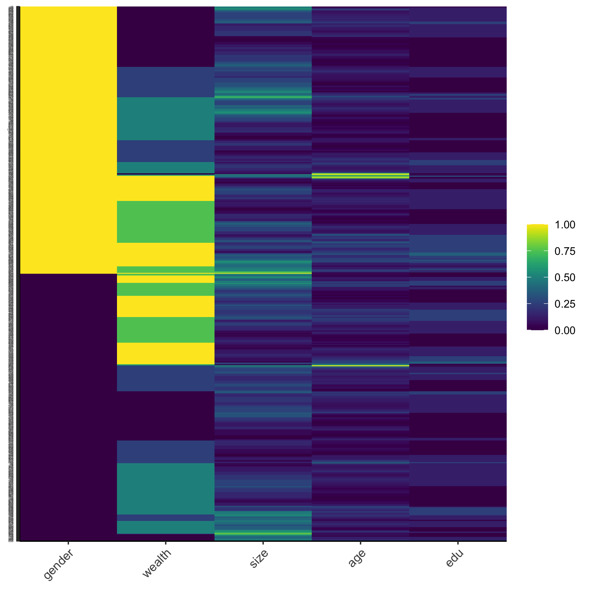
Percentized: