Project 2 - Zambia DHS Data Analysis and Modeling

I requested and obtained DHS data for Zambia (2018, DHS-VII).

Model 1 - Penalized Logistic Regression

Using the R script provided, split and sample your DHS persons data and evaluate the AUC - ROC values you produce. Which “top_model” performed the best (had the largest AUC)?

Below are the results of the “top_models”:

    penalty .metric .estimator  mean     n std_err .config              
      <dbl> <chr>   <chr>      <dbl> <int>   <dbl> <chr>                
 1 0.0001   roc_auc hand_till  0.608     1      NA Preprocessor1_Model01
 2 0.000127 roc_auc hand_till  0.608     1      NA Preprocessor1_Model02
 3 0.000161 roc_auc hand_till  0.608     1      NA Preprocessor1_Model03
 4 0.000204 roc_auc hand_till  0.608     1      NA Preprocessor1_Model04
 5 0.000259 roc_auc hand_till  0.608     1      NA Preprocessor1_Model05
 6 0.000329 roc_auc hand_till  0.608     1      NA Preprocessor1_Model06
 7 0.000418 roc_auc hand_till  0.608     1      NA Preprocessor1_Model07
 8 0.000530 roc_auc hand_till  0.608     1      NA Preprocessor1_Model08
 9 0.000672 roc_auc hand_till  0.608     1      NA Preprocessor1_Model09
10 0.000853 roc_auc hand_till  0.609     1      NA Preprocessor1_Model10
11 0.00108  roc_auc hand_till  0.608     1      NA Preprocessor1_Model11
12 0.00137  roc_auc hand_till  0.608     1      NA Preprocessor1_Model12
13 0.00174  roc_auc hand_till  0.607     1      NA Preprocessor1_Model13
14 0.00221  roc_auc hand_till  0.606     1      NA Preprocessor1_Model14
15 0.00281  roc_auc hand_till  0.603     1      NA Preprocessor1_Model15

Based on this output, model 10 had the largest AUC (0.609) and thus performed the best.

Are you able to use the feature selection penalty to tune your hyperparameter and remove any potentially irrelevant predictors? Provide justification for your selected penalty value.

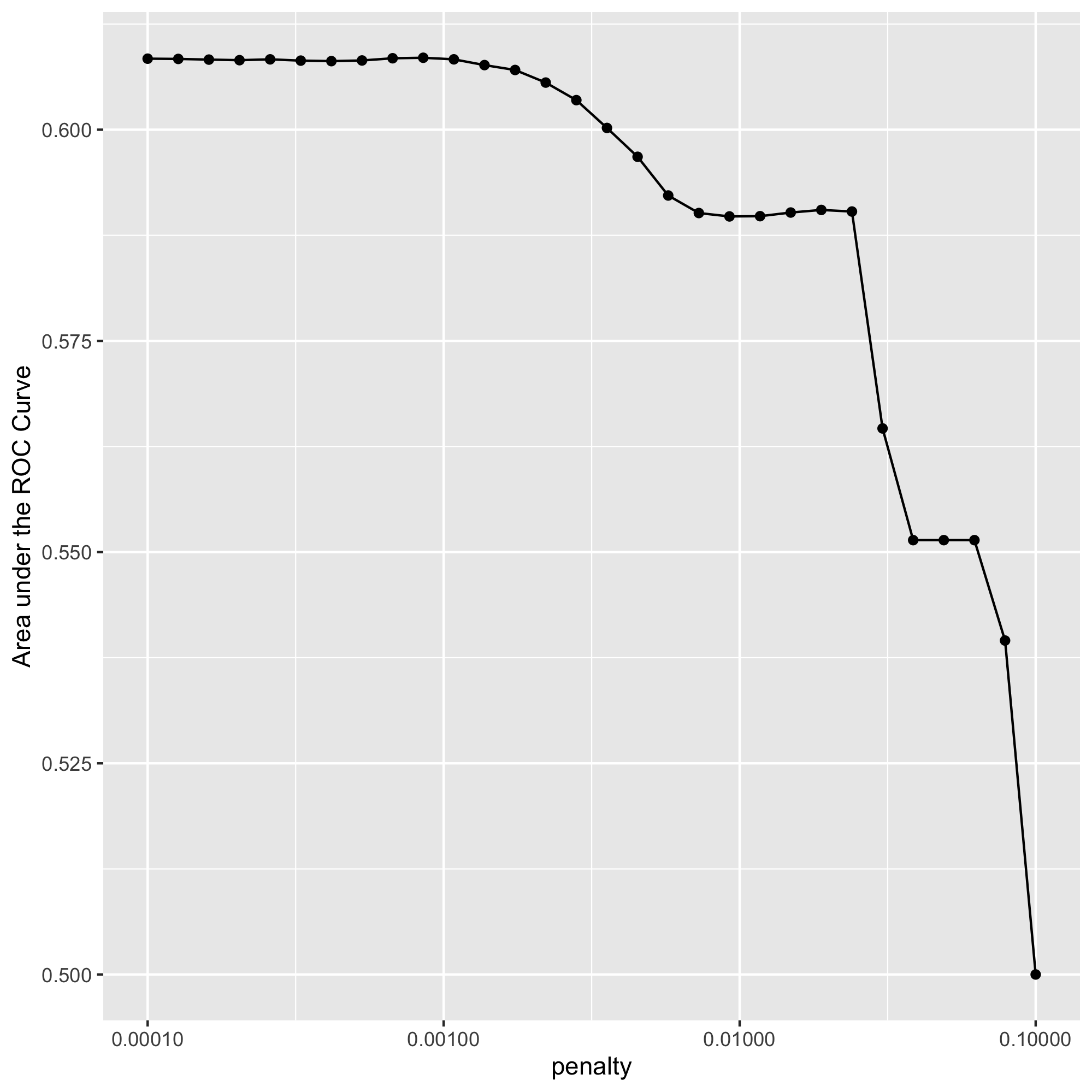
My selected penalty value is 0.000853. Looking at the “top_models” output, model 10 has the largest mean AUC, 0.609, with a penalty of 0.000853. Additionally, based on the penalty vs AUC plot above, AUC appears to begin to decrease after about model 10.

Finally, provide your ROC plots and interpret them. How effective is your penalized logistic regression model at predicting each of the five wealth outcomes?

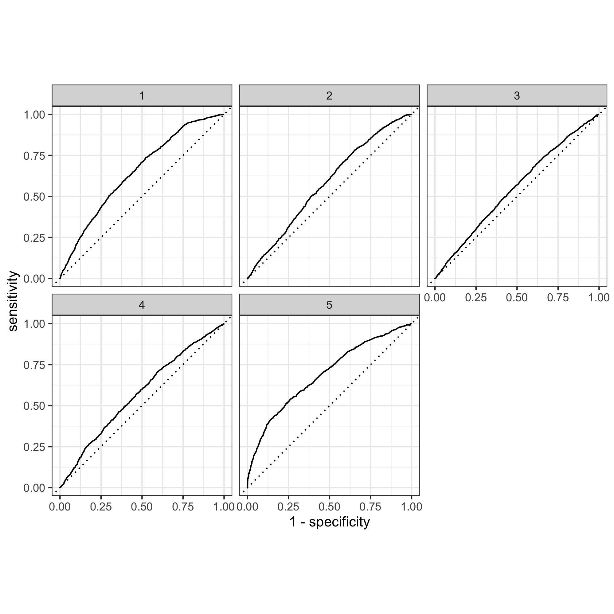
I used a penalty of 0.000853, or slice 10, for the ROC plots. To determine how effective the model is, we can look at how close the plot is to the 45 degree line; the closer to the straight line the worse the model is at predicting the wealth outcome versus the others. The penalized logistic regression is most effective at predicting wealth outcomes 1 and 5, and less effective at differentiating 2, 3, and 4 from the others. The model performed best when predicting wealth group 5, then 1. It seems to perform okay, but not well when predicting groups 2 and 4, but overall appears to not perform very well when differentiating between 2, 3, and 4, or the middle wealth outcomes.

Model 2 - Random Forest Model

Using the R script provided, set up your random forest model and produce the AUC - ROC values for the randomly selected predictors, and the minimal node size, again with wealth as the target.

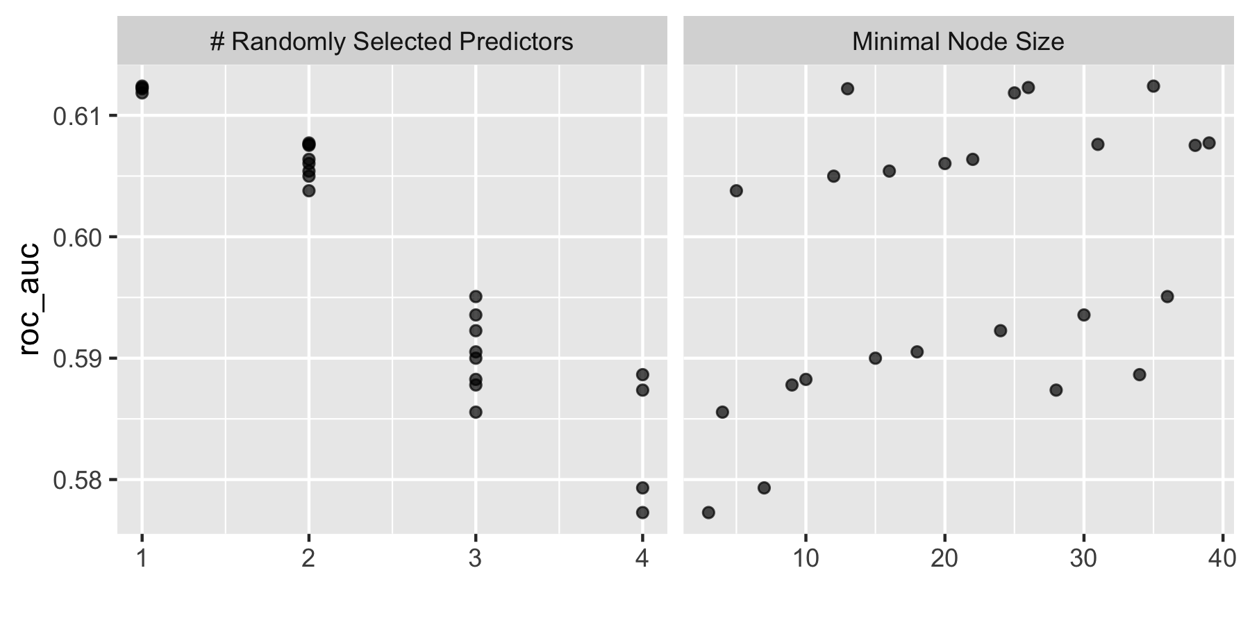
How did your random forest model fare when compared to the penalized logistic regression?

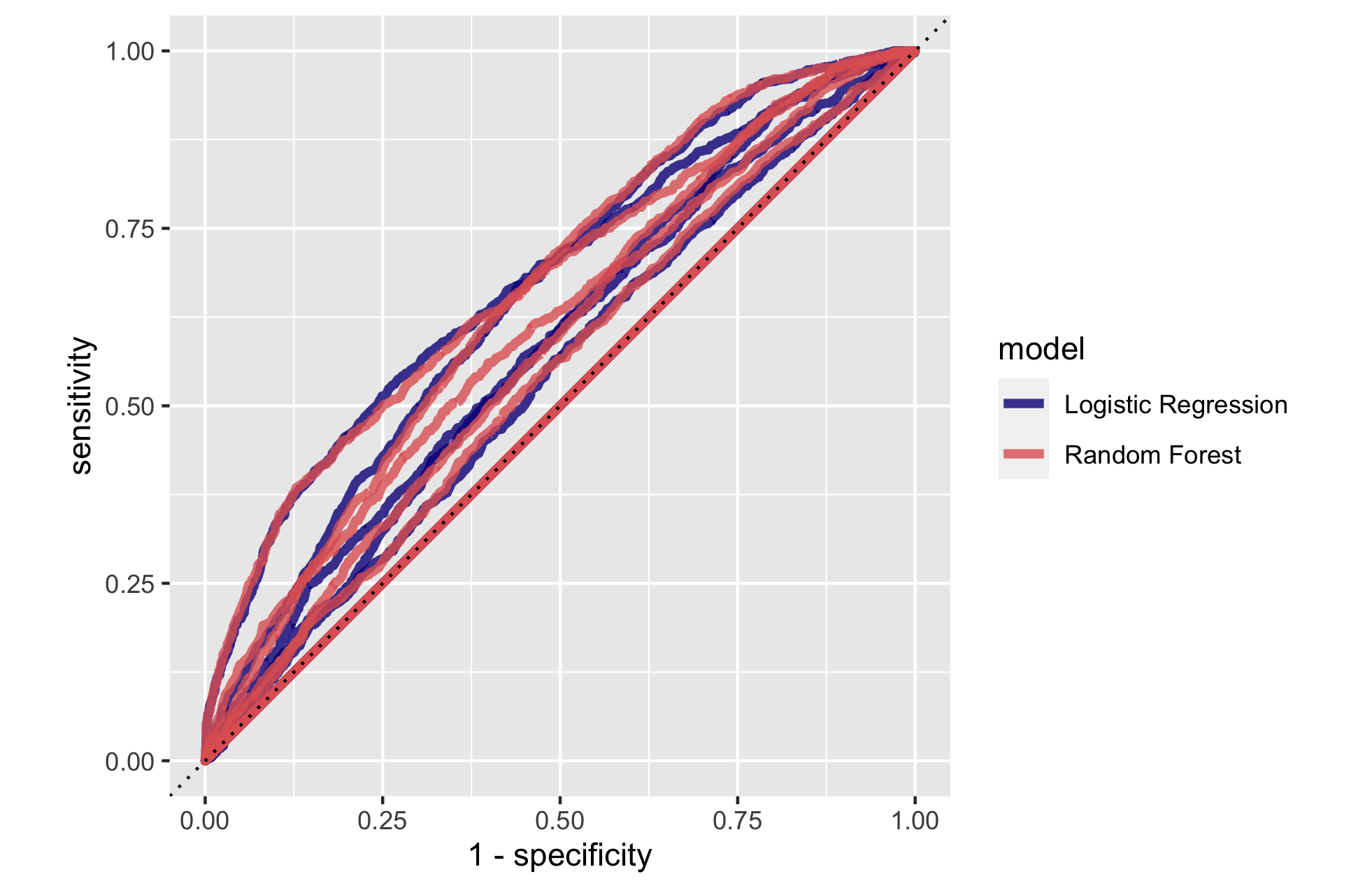
The random forest model is fairly comparable to the penalized logistic regression. It appears to perform a little better than the penalized logistic regression in some wealth outcomes, but overall the models performed similarly.

Provide your ROC plots and interpret them.

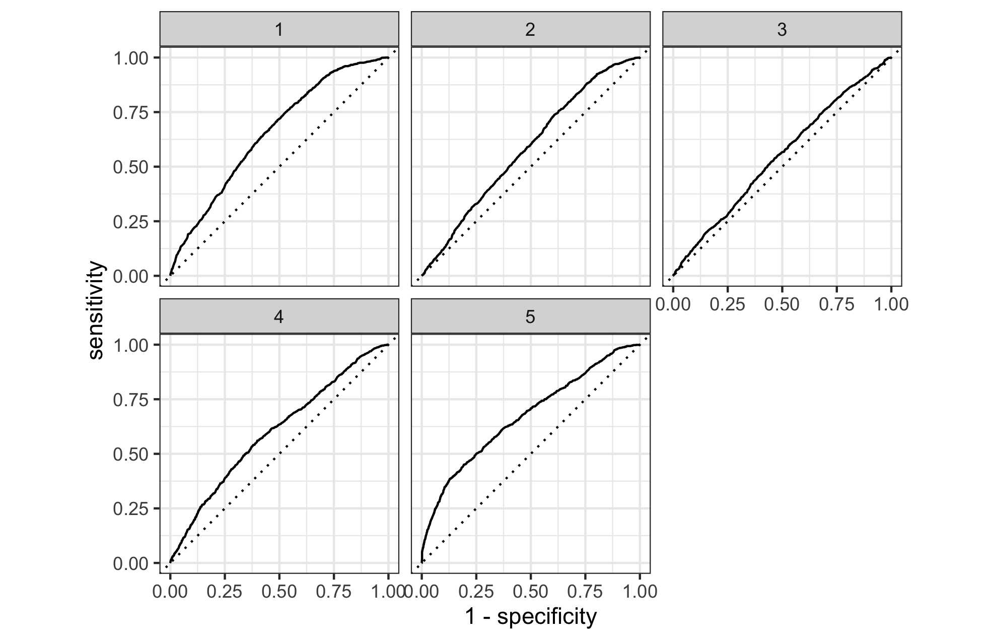
Similar to the penalized logistic regression, the random forest model is most effective at predicting wealth outcomes 1 and 5, and less effective at differentiating 2, 3, and 4 from the others. The model overall appears to not perform as well when differentiating between 2, 3, and 4 and the others, or the middle wealth outcomes. There does appear to perhaps be a small improvement in predicting the middle wealth outcomes versus the penalized logistic regression, but overall the models perform similarly.

Are you able to provide a plot that supports the relative importance of each feature’s contribution towards the predictive power of your random forest ensemble model?

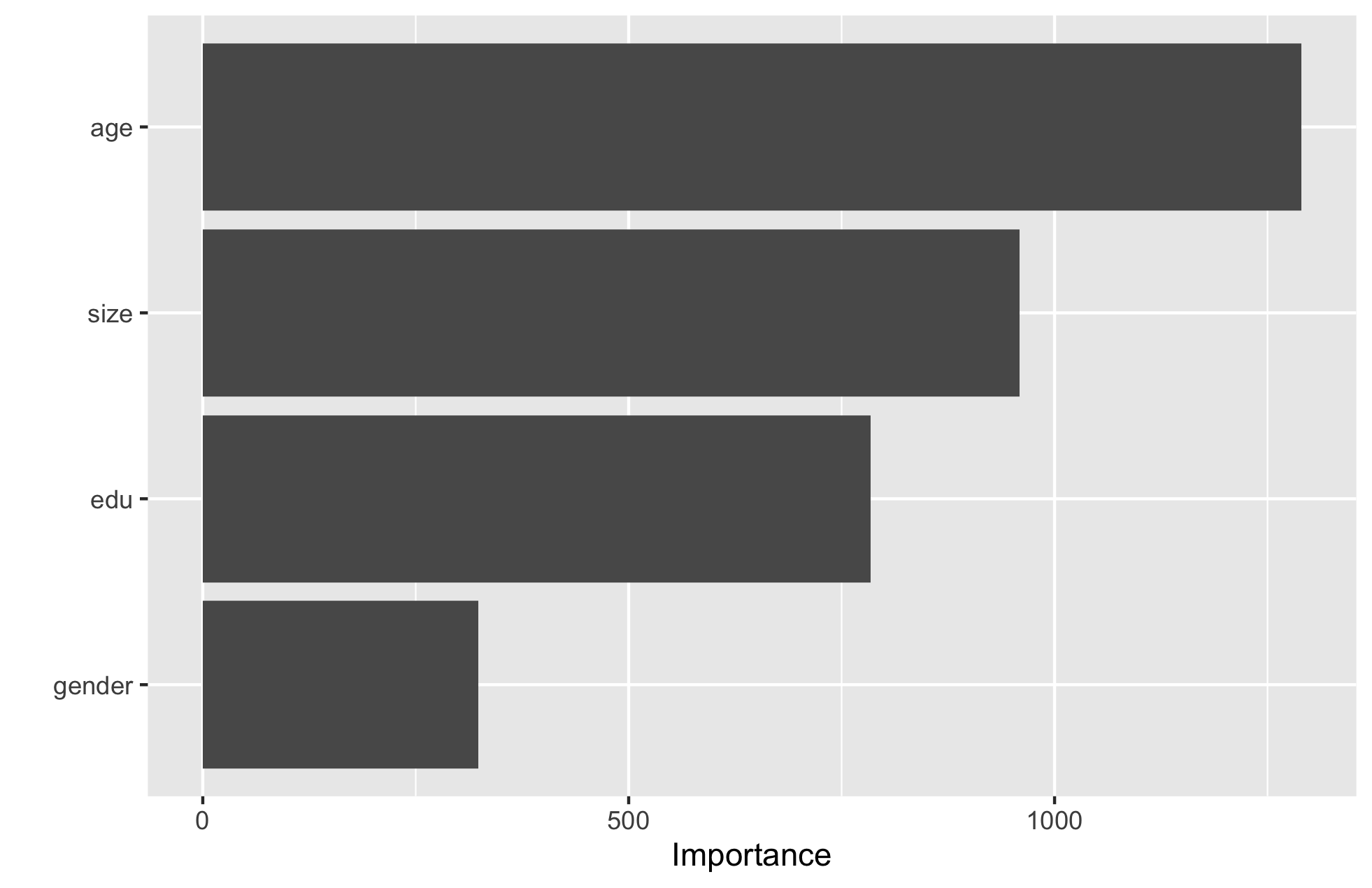
It appears that age is the most important feature in terms of contribution to predictive power, and gender is the least important. I would have guessed that perhaps education level would be of more importance, so that was a somewhat surprising outcome. It would be interesting to look at other features of the data.

Model 3 - Logistic Regression Model

Using the python script provided, train a logistic regression model using the tensorflow estimator API and your DHS data, again with wealth as the target. Apply the linear classifier to the feature columns and determine the accuracy, AUC and other evaluative metrics towards each of the different wealth outcomes.

Evaluative Metric	Result (wealth 1)	Result (wealth 2)	Result (wealth 3)	Result (wealth 4)	Result (wealth 5)
accuracy	0.776949	0.781069	0.784110	0.827759	0.819225
accuracy_baseline	0.776949	0.781069	0.784110	0.827759	0.819225
auc	0.631950	0.535903	0.536906	0.564764	0.649596
auc_precision_recall	0.295410	0.232036	0.236950	0.210365	0.309374
average_loss	0.510198	0.522409	0.520388	0.456083	0.443171
label/mean	0.223051	0.218931	0.215890	0.172241	0.180775
loss	0.510198	0.522409	0.520388	0.456083	0.443171
precision	0.000000	0.000000	0.000000	0.000000	0.000000
prediction/mean	0.223939	0.225920	0.219684	0.169870	0.180851
recall	0.000000	0.000000	0.000000	0.000000	0.000000
global_step	100.000000	100.000000	100.000000	100.000000	100.000000

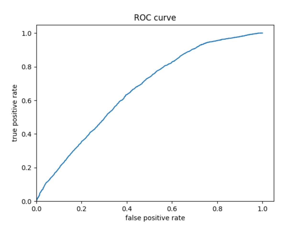
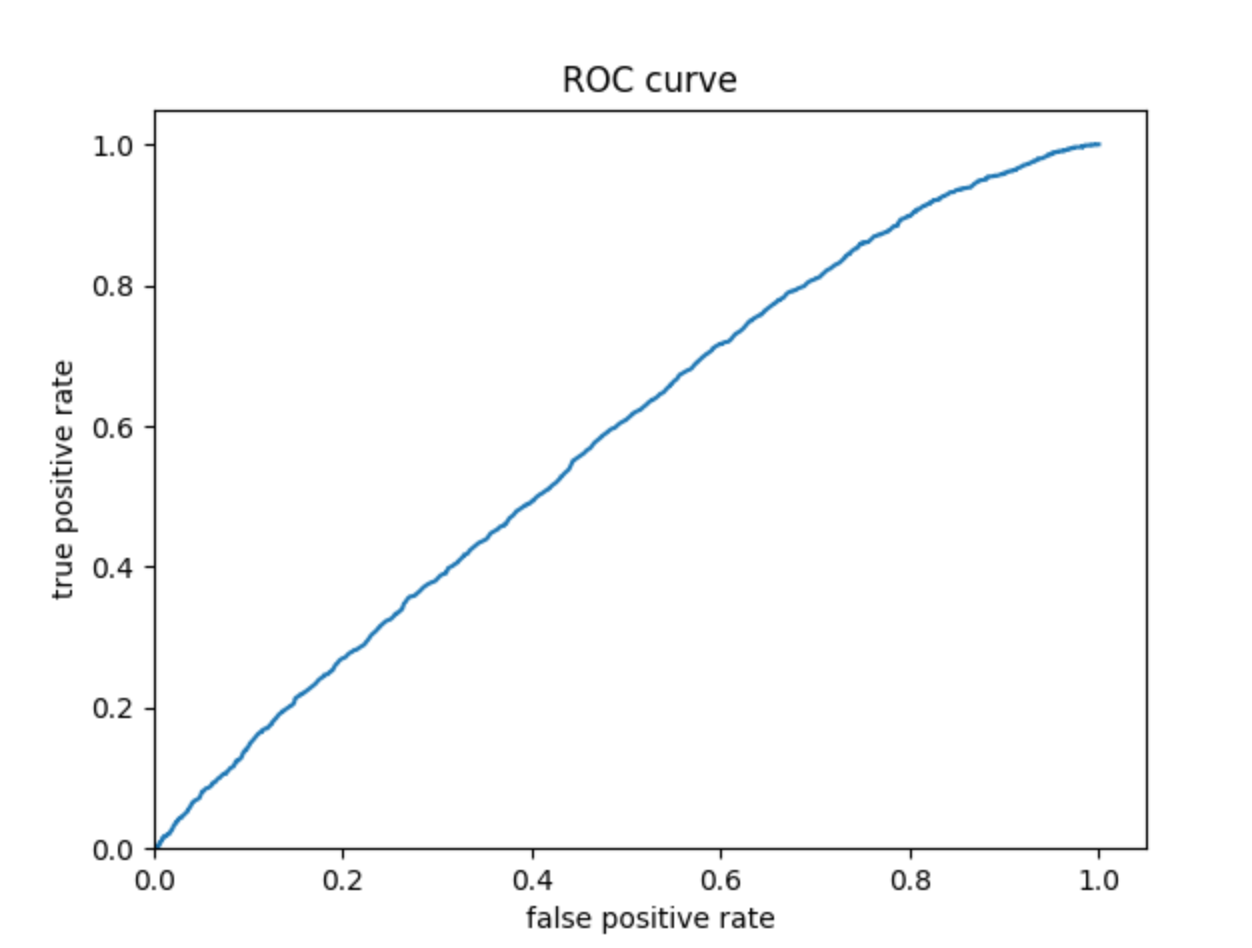
Then continue with your linear classifier adding the derived feature columns you have selected in order to extend capturing combinations of correlations (instead of learning on single model weights for each outcome). Again produce your ROC curves and interpret the results.

Wealth 1:

Wealth 2:

Wealth 3:

Wealth 4:

Wealth 5:

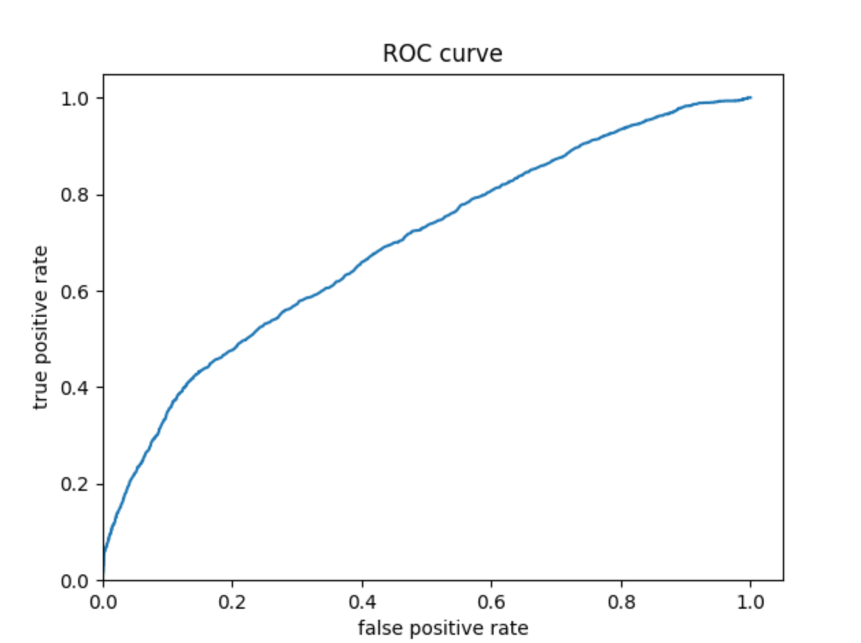
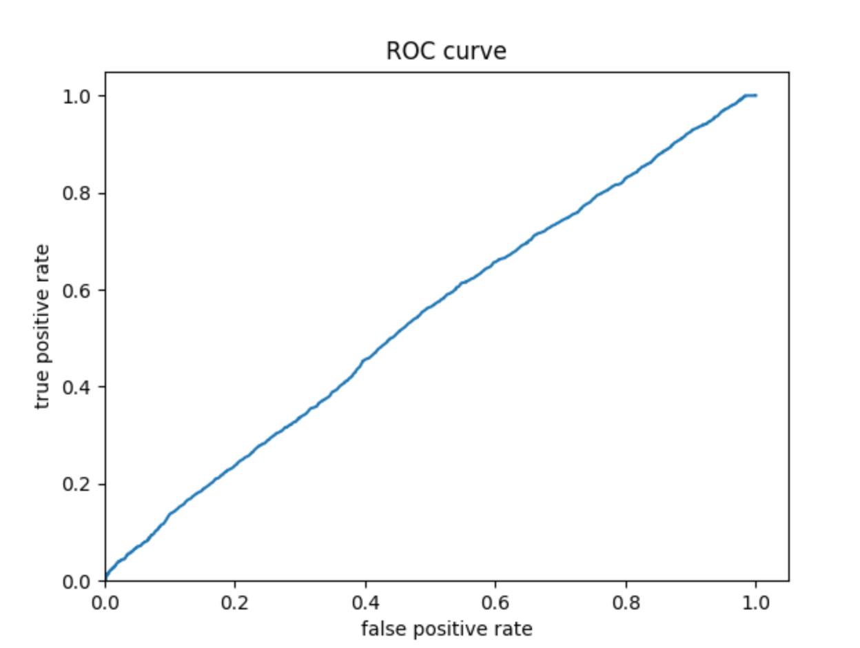
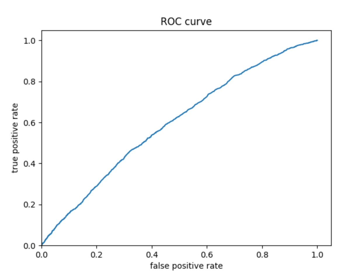
The ROC curves for the logistic regression model are similar to those of the penalized logistic regression and random forest models; the model performs better and has a larger AUC for wealth 1 and 5. The model is not very effective at differentiating wealths 2, 3, and 4. Similar to the previous models, this model does perhaps predict wealth 4 a bit better than wealths 2 and 3.

Model 4 - Gradient Boosting Model

Using the python script provided, train a gradient boosting model using decision trees with the tensorflow estimator. Provide evaluative metrics including a measure of accuracy and AUC.

Evaluative Metric	Result (wealth 1)	Result (wealth 2)	Result (wealth 3)	Result (wealth 4)	Result (wealth 5)
accuracy	0.777440	0.780284	0.784306	0.828543	0.826974
accuracy_baseline	0.776949	0.785875	0.784110	0.827759	0.819225
auc	0.654496	0.659469	0.549197	0.607277	0.689823
auc_precision_recall	0.326235	0.319574	0.251778	0.249540	0.378418
average_loss	0.500891	0.487646	0.516750	0.448407	0.430754
label/mean	0.223051	0.214125	0.215890	0.172241	0.180775
loss	0.500891	0.487646	0.516750	0.448407	0.430754
precision	0.575758	0.571429	0.545455	0.681818	0.739394
prediction/mean	0.219308	0.219959	0.215268	0.164324	0.177925
recall	0.008355	0.003665	0.005452	0.008542	0.066196
global_step	100.000000	100.000000	100.000000	100.000000	100.000000

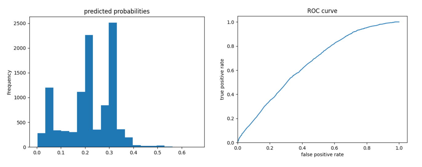
Produce the predicted probabilities plot as well as the ROC curve for each wealth outcome and interpret these results.

Wealth 1:

Wealth 2:

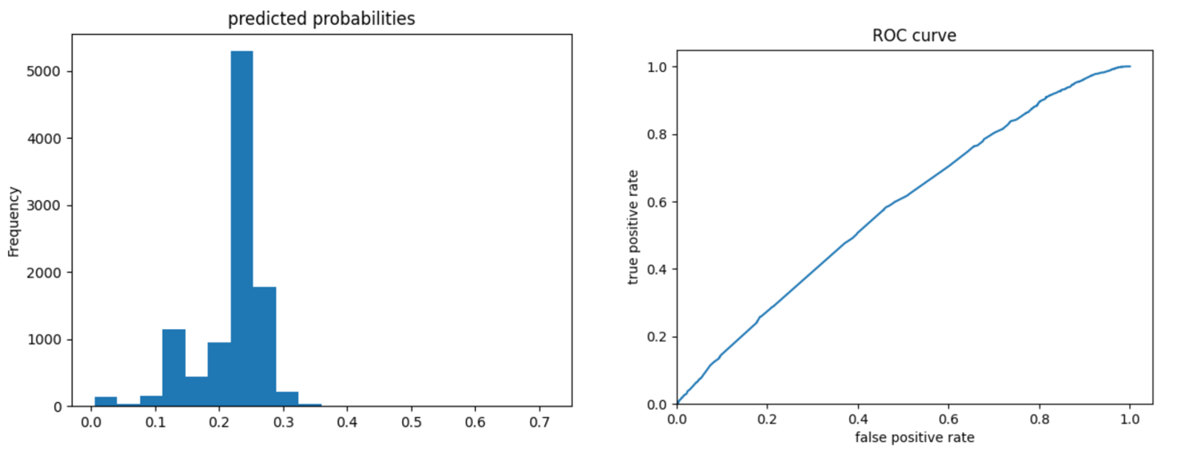
Wealth 3:

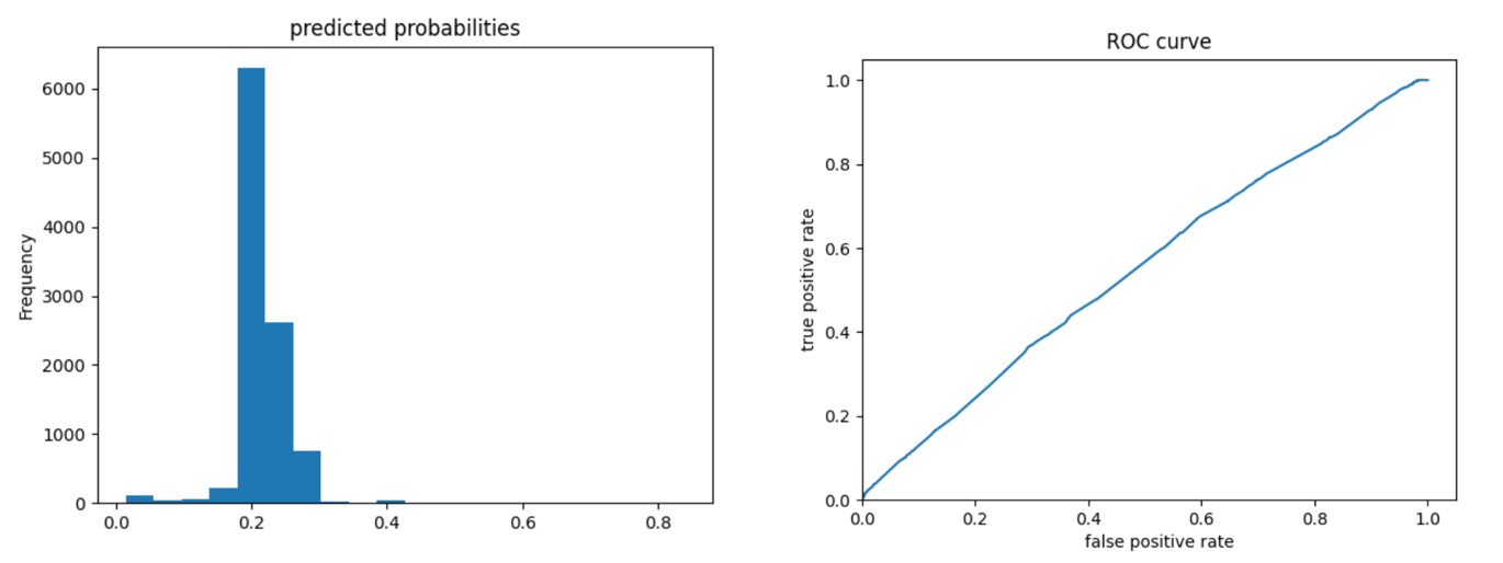
Wealth 4:

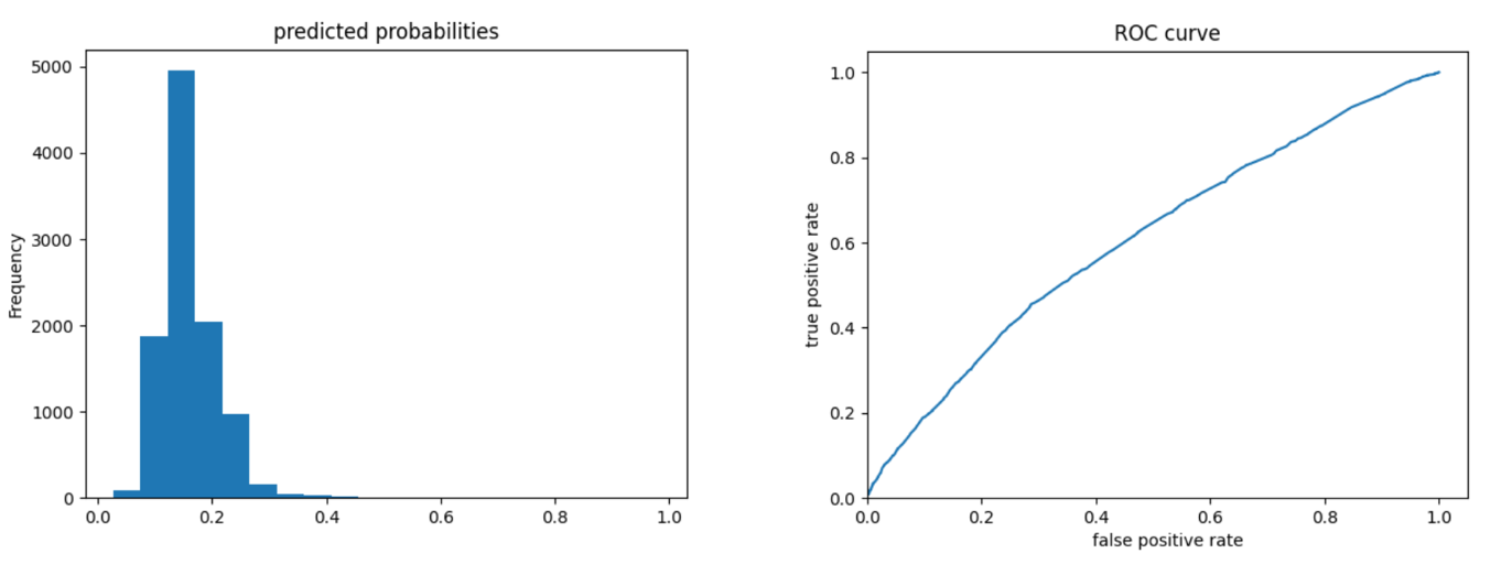
Wealth 5:

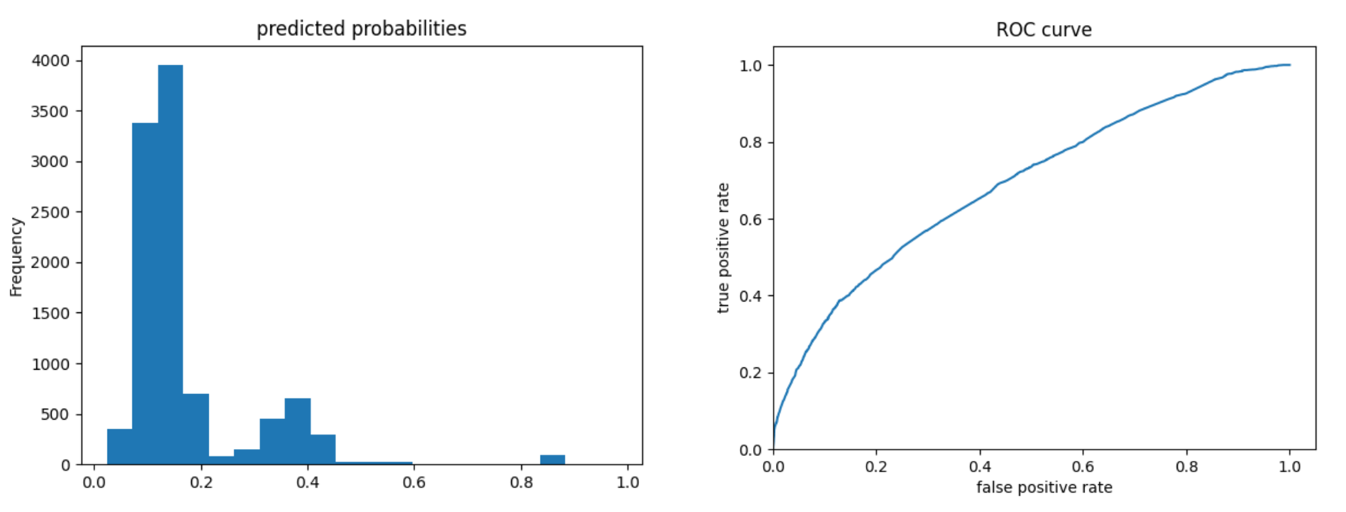
The ROC curves for the gradient boosting model are again pretty similar to those of previous models; the model performs better and has a larger AUC for wealth 1 and 5. The model is not as effective at differentiating wealths 2, 3, and 4 from the others. Compared to the logistic regression model, we can look at the evaluative metrics and see that the gradient boosting model overall appears to have slightly improved accuracy and also outputs a slightly larger AUC for all wealths - particularly for wealths 2 and 4.

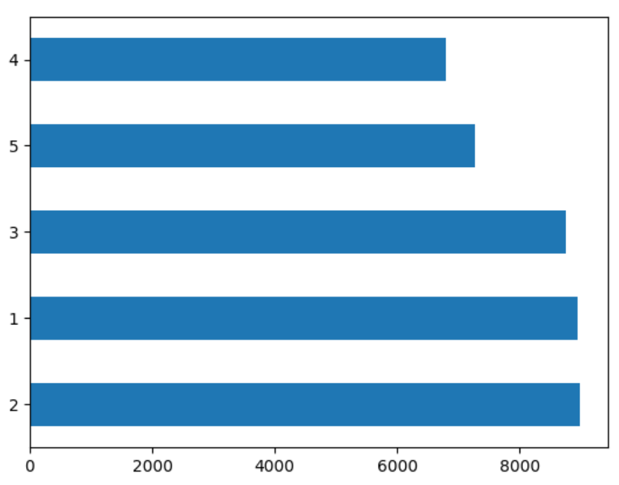
Looking at the predicted probabilities plots, these outcomes make sense because there is a larger number of people in wealth outcomes 1-3 than 4 and 5, so the predictive probabilities would be higher for those wealth outcomes.

Analyze all four models

According to the evaluation metrics, which model produced the best results? Were there any discrepancies among the five wealth outcomes from your DHS survey dataset?

According to the evaluation metrics, the gradient boosting model produced the best results. It had a higher accuracy across the wealth outcomes, and also had the larger AUC for the wealth outcomes. The four models performed similarly - they performed better when predicting the “extremes” of the wealth category, wealths 1 and 5. Model performance was not as good for the middle wealth outcomes.